python

Finalytics is a portfolio analytics engine written in Rust, with this typed Python package over it. It compares portfolio optimisation methods on returns they have not seen, keeps the books of a real portfolio to report its performance, risk and attribution, tests a plan's chance of meeting a goal, and screens thousands of securities by rules on their measures.

pip install "finalytics[pandas]"  # with pandas, as the examples below use
pip install finalytics            # with NumPy only

Without pandas, the datasets come as price tables, which Assets takes as well: fl.Assets(fl.datasets.asset_class_table(), risk_free_asset="T-Bills").

Until 1.0.0 is released, pip install finalytics gives 0.9; install a 1.0 pre-release with pip install --pre finalytics. The migration guide explains what replaces each part of 0.9.

Sample reports, built by the programs below from the bundled datasets and, for screening, the S&P 500 prices in tests/sp500: comparison · backtest · optimisation · portfolio · rebalance · planning · screening

Portfolio optimisation

Compare optimisation methods on the same assets. Each method is refitted every quarter on the five years before, and judged on the quarter that follows.

import finalytics as fl

assets = fl.Assets(fl.datasets.asset_class_prices(), risk_free_asset="T-Bills")

result = assets.compare(
    methods=[
        "equal_weight",
        "minimum_variance",
        "maximum_sharpe",
        "maximum_diversification",
        "risk_parity",
        "hierarchical_risk_parity",
    ],
    max_weight=0.40,
    rebalance="quarterly",
    validation=fl.WalkForward(years=5),
    trading_cost_bps=10,
)

result.show()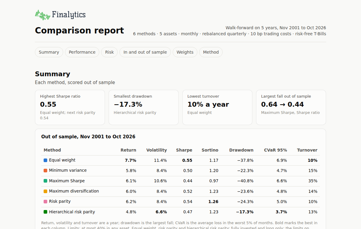

Every result has the same shape: result.report is the report, which print(result) prints as text and result.show() opens as a page (inline in a Jupyter notebook), and result.results holds every return and trade behind it. A program that shows pages itself, such as a web page running Python with Pyodide, hands show() a function with fl.set_show_handler, which then receives each page's HTML.

To test one allocation, give a method or your own weights. Here, the maximum Sharpe ratio fitted to the years before November 2016, held from then on against a 60/40 benchmark:

result = assets.backtest(
    method="maximum_sharpe",
    max_weight=0.40,
    benchmark={"US Equity": 0.60, "Bonds": 0.40},
    rebalance="quarterly",
    validation=fl.Holdout(start="2016-11-01"),
)

result.show()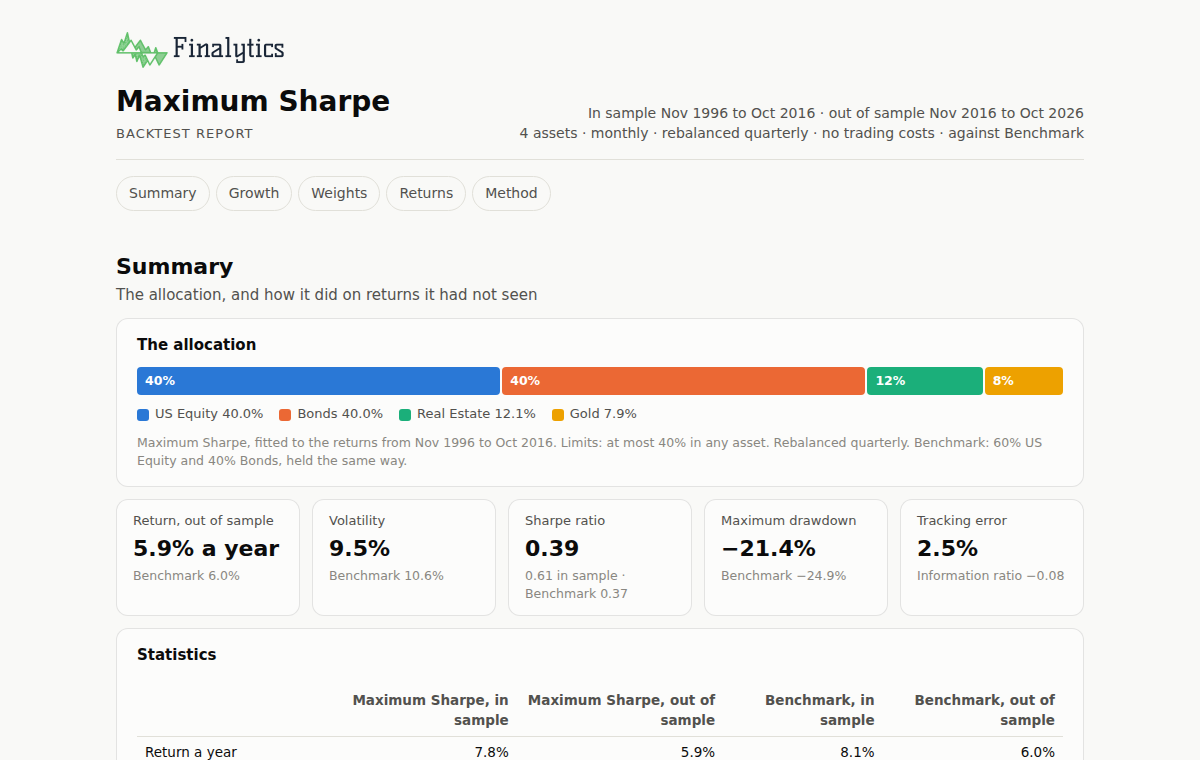

To see the weights a method chooses today, where their risk comes from and where they sit on the efficient frontier:

result = assets.optimise(
    method="maximum_sharpe", max_weight=0.40, frontier=True
)

result.show()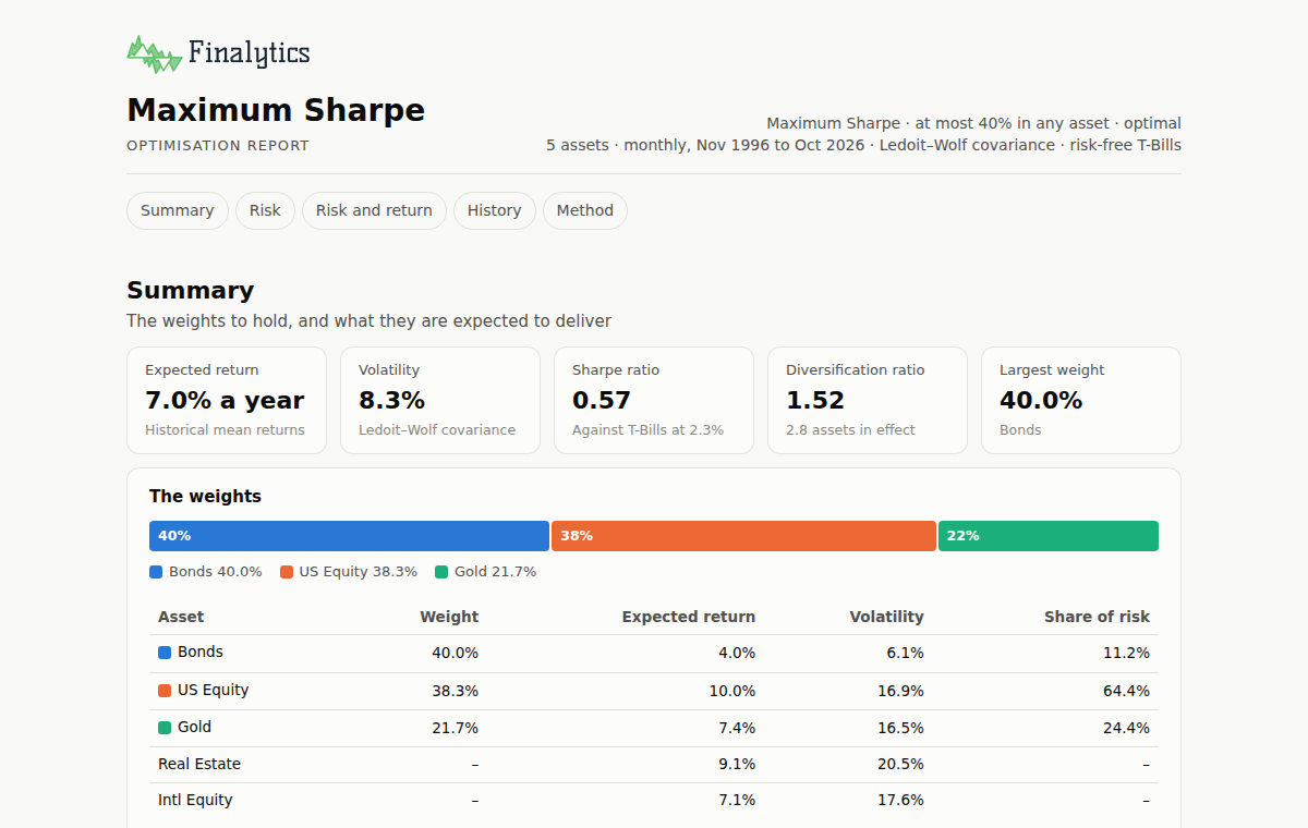

Portfolio analytics

Load a portfolio from its transactions and prices, and report on it: holdings, performance, risk, attribution and scenarios.

import finalytics as fl

portfolio = fl.Portfolio.from_csv(
    transactions="transactions.csv",
    prices="prices.csv",
    fx="fx.csv",
    instruments="instruments.csv",
    accounts="accounts.csv",
)

report = portfolio.report(benchmark="BENCH", group_by=["asset_class", "region"])

report.show()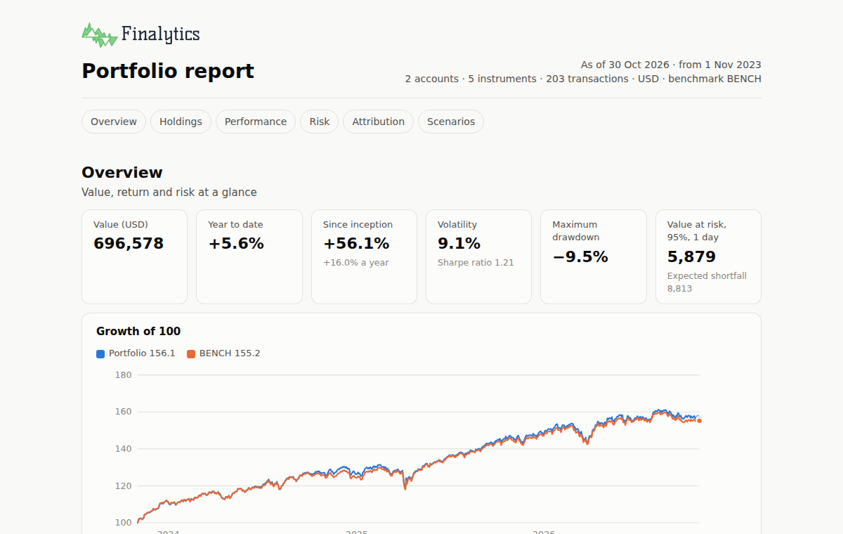

The files are the portfolio dataset: a household's brokerage and retirement accounts, holding five funds in dollars and euros for three years. fl.datasets.file("portfolio/prices.csv") and the like return each of them, and fl.datasets.portfolio() loads the same portfolio without them. BENCH is a column of prices.csv, the benchmark's levels; asset_class and region are columns of instruments.csv that classify each holding. The sample report adds the attribution and scenarios of fl.datasets.report_options(). A portfolio's report is its own result: every figure in it is the portfolio's, so report() returns the report, with no results beside it.

The start of the dataset's files

id,kind,currency,name,class.asset_class,class.region
VTI,fund,USD,Vanguard Total Stock Market ETF,Equity,North America
EXSA,fund,EUR,iShares STOXX Europe 600 UCITS ETF (DE),Equity,Europe

date,VTI,EXSA,BND,GLD,VNQ,BENCH
2023-11-01,208.86,43.21,68.99,183.51,73.37,100.0000
2023-11-02,213.01,43.92,69.39,184.12,75.78,101.4345

id,name,lot_method,taxable,class.owner,class.wrapper
brokerage,Brokerage account,fifo,true,Alex,Taxable
ira,Retirement account,fifo,false,Alex,Tax-deferred

The data guide describes every file, column by column.

To move the same funds to their least risky mix, 5% to 40% each, optimise the holdings and rebalance the accounts together, with fees and tax rates:

target = portfolio.assets().optimise(
    method="minimum_variance", bounds=(0.05, 0.40)
)

result = portfolio.rebalance(
    target, whole_units=True, fee_bps=5, minimum_fee=1, tax=(0.37, 0.20)
)

result.show()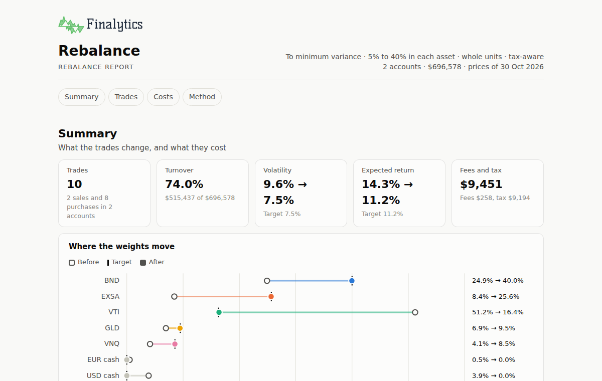

Sales in the brokerage account take the lots that cost the least tax; the retirement account is not taxable (taxable is false in accounts.csv), so its sales pay none. portfolio.with_rebalance(result) makes the trades.

Financial Planning

Test a plan of saving, spending and investing against one goal: an amount by a date, such as a house deposit, or payments over a period, such as an income in retirement. The plan runs month by month through 10,000 markets drawn from the assets' monthly returns, in today's money: returns are after inflation and fees.

import finalytics as fl

assets = fl.Assets(fl.datasets.asset_class_prices())

plan = assets.plan(
    fl.Payments(amount=4_000, start="2046-11", end="2076-10"),
    name="Retirement income",
    chance=0.85,
    start_value=250_000,
    flows=[fl.Saving(amount=1_500, every="month")],
    weights=("Balanced 60/40", {"US Equity": 0.60, "Bonds": 0.40}),
    alternatives={
        "Cautious 30/70": {"US Equity": 0.30, "Bonds": 0.70},
        "Growth 80/20": {"US Equity": 0.80, "Bonds": 0.20},
    },
    inflation=0.025,
    fee=0.0025,
    currency="USD",
)

plan.show()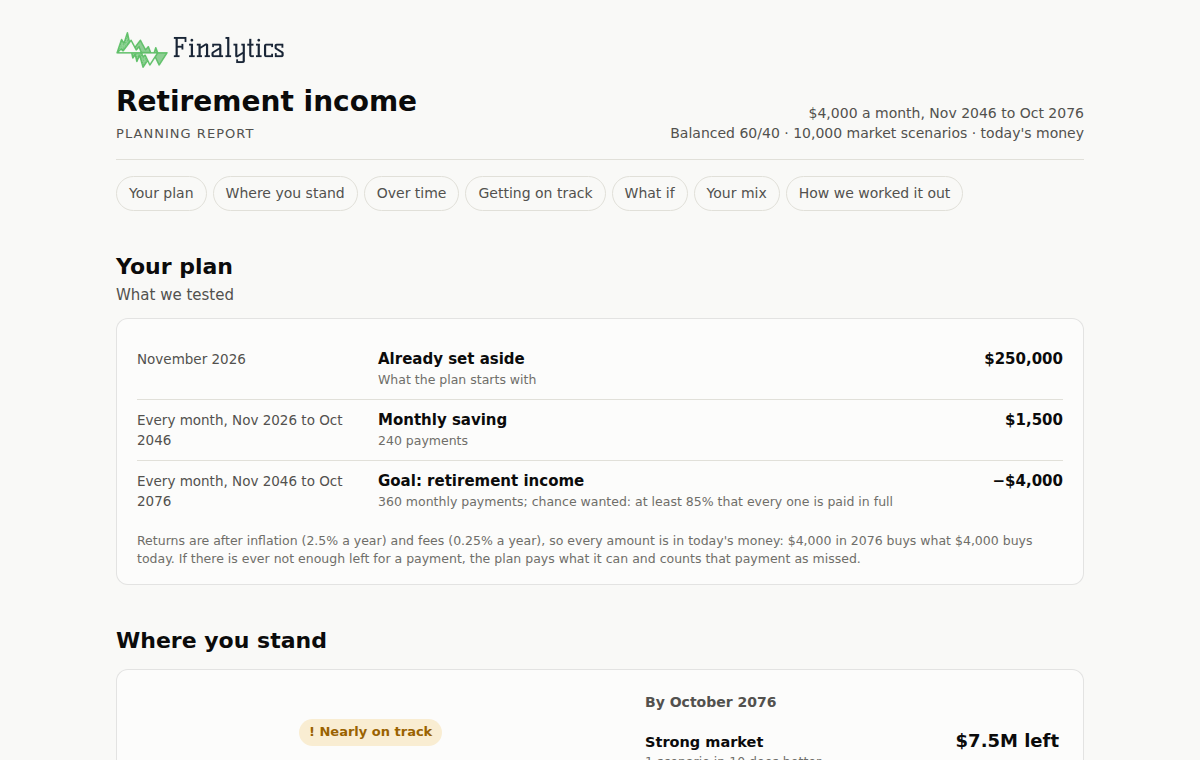

The report gives the chance of meeting the goal against the chance wanted, how the money could grow, and the smallest change that would reach that chance: saving more, starting with more, starting the payments later or taking a little less. It tests the plan when returns are lower and when markets crash as the payments start, and compares other mixes on the same simulations. plan.results holds the figures behind it, with the value over time.

For an amount by a date, give fl.Target(amount=150_000, by="2030-06"); for a single payment out along the way, fl.Spending(name="Car", amount=25_000, on="2028-03"); and for inflation month by month, a price index of one column, such as a consumer price index, inflation=index.

Screening

Screen many securities at once, each measured on its own history: returns over calendar windows, risk, measures against a benchmark, technical indicators, income and volume. Rules test the measures and any fields given with the securities, such as a sector or a price-to-earnings ratio.

import finalytics as fl

universe = fl.Universe(
    "tests/sp500/prices.csv",
    fields="tests/sp500/companies.csv",
    risk_free_rate=0.04,
)

screen = universe.screen(
    rules=[
        ("return_1y", ">", 0.0),
        ("volatility", "<", 0.30),
        ("price_to_sma_200", ">", 1.0),
        ("rsi_14", "between", (30, 70)),
        ("max_drawdown_3y", ">", -0.30),
        ("sector", "not_in", ["Utilities"]),
    ],
    sort=("sharpe_ratio_3y", "descending"),
    limit=10,
)

screen.show()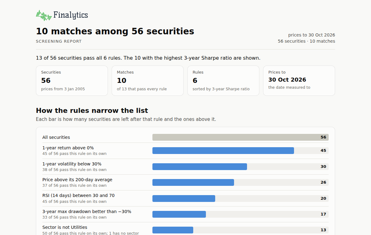

The report shows how the rules narrow the list, the matches in order, the near misses and where each rule's threshold falls across the universe.

What is included

Optimisation

• Equal weight, minimum variance, mean–variance and robust mean–variance, maximum Sharpe, target return or volatility, maximum diversification, minimum CVaR, risk parity, hierarchical risk parity
• Limits on each asset and on groups, turnover, tracking error and factor exposure
• Black–Litterman and resampled estimates; Ledoit–Wolf, OAS and EWMA covariance
• Validation in sample, on a holdout, or walk-forward; calendar or drift rebalancing; trading costs

Analytics

• Books from transactions: lots, corporate actions, several accounts and currencies
• Time- and money-weighted returns, contribution, Brinson–Fachler and currency attribution
• Volatility, drawdowns, value at risk, risk decomposition, factor models and scenarios
• Rebalancing trades with fees and tax-aware lot selection, across accounts

Planning

• The chance of a goal, an amount by a date or payments over a period, from simulated markets: block bootstrap, normal or historical
• Saving and spending once or regularly, fixed or glide-path mixes, fees and inflation, in today's money
• The changes that reach the chance wanted, lower returns and a crash, and other mixes on the same simulations

Screening

• Thousands of securities, each on its own dates, with volumes, dividends and fields such as a sector or a valuation
• Returns over calendar windows, volatility, drawdowns, Sharpe and Sortino ratios, value at risk, beta and relative returns, moving averages, RSI and MACD, dividend yield and volume
• Rules on the measures and on the fields, sorted and limited

Every report prints as text, 80 columns wide, and shows as one self-contained HTML page, in light and dark. Every model is tested against an independent implementation; the methods pages define each one.

Beneath the front doors, fl.risk, fl.opt and fl.performance give each method on its own, and results are frozen dataclasses with documented fields (see finalytics.types). Wheels are published for Linux, macOS and Windows.

Documentation

Data guide · Methods · Performance · Migrating from 0.9 · Source and issues

Contributing and licence

Contributions are welcome: see CONTRIBUTING.md. Finalytics is licensed under MIT or Apache-2.0, at your option. It provides analysis tools only and is not investment advice.