Scientific Machine Learning - Peking Module

Lecture notes, Julia demonstrations, notebooks, assignments, and generated figures for a scientific machine learning study module.

Overview

This repository collects the materials used while studying scientific machine learning with a Julia-based workflow. The content starts with Julia programming fundamentals, then moves into plotting, linear and nonlinear systems, and numerical optimization.

Core topics include:

• Julia syntax, arrays, functions, types, and basic scripting.
• Plotting and numerical visualization with CairoMakie and Plots.
• Linear systems, nonlinear equations, Newton-Raphson iterations, and contour analysis.
• Optimization workflows, including gradient-based and second-order methods.
• Linear least-squares modeling with gradient descent and normal equations.
• Differentiation in Julia and forward-mode automatic differentiation.
• Coursework artifacts, homework notebooks, CSV data, and lecture PDFs.

Repository Structure

Path	Contents
Chapter01/	Introduction, Julia basics, plotting, and equation-solving materials organized into Jupyter Notebooks, PDFs, and Julia.
Chapter02/	Optimization materials organized into Jupyter Notebooks, PDFs, and Julia, including gradient-based and second-order methods.
Chapter03/	Linear least-squares materials organized into Jupyter Notebooks, PDFs, and Julia.
Chapter04/	Differentiation, forward-mode automatic differentiation, and parameter estimation materials organized into Jupyter Notebooks, PDFs, and Julia.
Chapter05/	Boundary value problem materials (finite differences, nonlinear BVPs, inverse/parameter-estimation problems) organized into Jupyter Notebooks, PDFs, and Julia.
Chapter06/	Neural network materials, from a hand-built single neuron up to Lux-based multivariate networks and NN+physics models, organized into Jupyter Notebooks, PDFs, and Julia.
class 2/ / class 3/	Raw in-class live-coding demos (linear/nonlinear solving, plotting, gradient descent/momentum) that led up to the Day02/Day03 homework; mostly superseded by the polished Chapter01/Chapter02 material.
Assignment 1/, Assignment 2/	Assignment PDFs, solution scripts, and supporting CSV data.
Homework/	One subfolder per class day (Day02 … Day12), each with its handout PDF (where checked in) plus the matching solution script/notebook and data/figures.
Archive/	Superseded/incomplete scratch scripts kept for reference.
JuliaPrograms/	Introductory Julia program examples.

For a study-oriented navigation guide, see COURSE_INDEX.md. For an exam-prep index organized by problem type (which file to crib from, and what to change if the question differs), see PROBLEM_INDEX.md.

Visual Overview

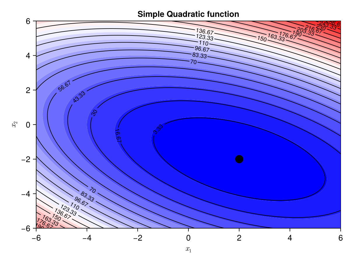
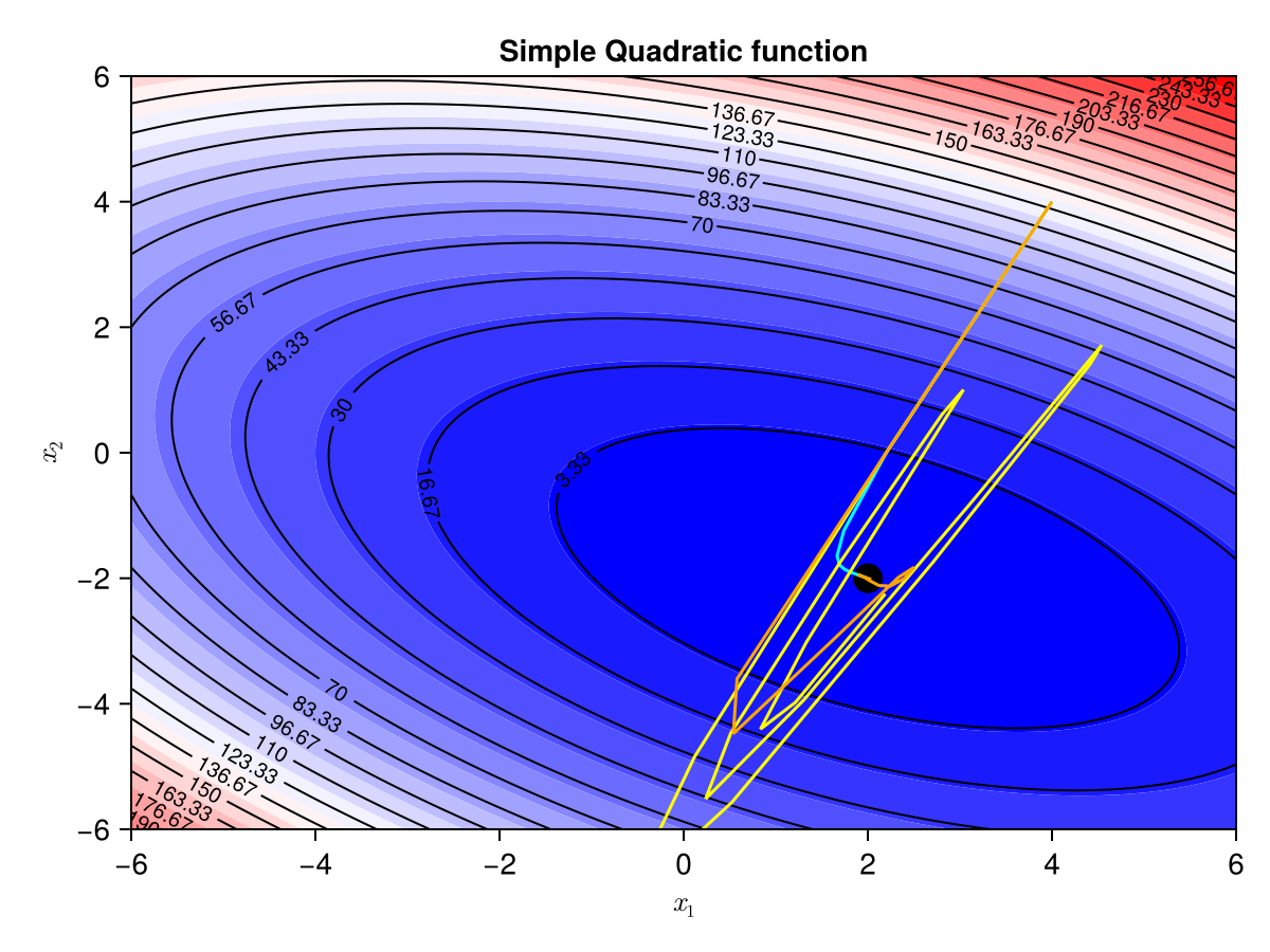
Optimization landscape	Algorithm comparison	Rosenbrock valley

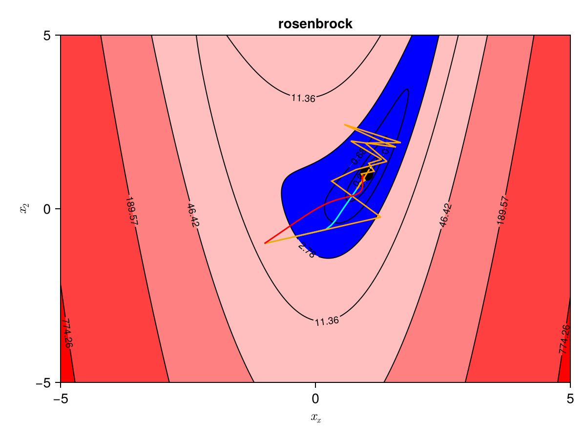These notebook-derived figures give the repository a more scientific visual summary: objective landscapes, contour geometry, and optimizer trajectories for gradient-based methods.

Getting Started

Install the local tools first:

• Julia for running scripts and notebooks.
• Visual Studio Code with the Julia extension, which provides the integrated REPL, plot pane, code completion, debugging, and Julia workspace tools.
• The Jupyter extension for VS Code for .ipynb notebook editing and execution. The extension also installs its common notebook helper extensions, including Jupyter Keymap, Notebook Renderers, Cell Tags, and Slide Show support.

Install the recommended VS Code extensions from PowerShell:

code --install-extension julialang.language-julia
code --install-extension ms-toolsai.jupyter

Download the Julia packages for the repository environment from the repository root:

julia --project=. -e "using Pkg; Pkg.instantiate()"

The same setup can also be run from the Julia REPL:

using Pkg
Pkg.activate(".")
Pkg.instantiate()

The class 2/ folder has its own Julia environment snapshot. Instantiate it separately when running those examples:

julia --project="class 2" -e "using Pkg; Pkg.instantiate()"

Run selected scripts from PowerShell:

julia "Chapter01\Julia\01p02.jl"
julia "class 2\nonlinear.jl"
julia "class 3\classdemo3.jl"

Open notebooks directly in VS Code, Jupyter, or another Julia-compatible notebook environment:

Chapter02/Jupyter Notebooks/02p01BasicOptimizationInJulia.ipynb
Chapter03/Jupyter Notebooks/03p02LinearLeastSquaresNormalEquations.ipynb

Main Dependencies

The Julia environment is defined in Project.toml and Manifest.toml. Major packages include:

• CairoMakie and Plots for visualization.
• LinearSolve and NonlinearSolve for equation solving.
• Optim, Optimization, OptimizationOptimJL, and OptimizationOptimisers for numerical optimization.
• ForwardDiff and Zygote for automatic differentiation.
• CSV and DataFrames for tabular data workflows.

For environment setup and generated-output notes, see REPRODUCIBILITY.md.

Notes

• Lecture materials are stored as PDFs for reference and review.
• Notebooks may be larger than the scripts because they can include embedded outputs.
• The Peking University seal is included from Wikimedia Commons, which identifies the original source as pku.edu.cn and notes that trademark or insignia restrictions may apply.